Multiplier (economics)

In macroeconomics, a multiplier is a factor of proportionality that measures how much an endogenous variable changes in response to a change in some exogenous variable.

For example, suppose variable x by 1 unit, which causes another variable y to change by M units. Then the multiplier is M.

Common uses

Two multipliers are commonly discussed in introductory macroeconomics.

Money multiplier

In monetary microeconomics and banking, the money multiplier measures how much the money supply increases in response to a change in the monetary base.

The multiplier may vary across countries, and will also vary depending on what measures of money are considered. For example, consider M2 as a measure of the U.S. money supply, and M0 as a measure of the U.S. monetary base. If a $1 increase in M0 by the Federal Reserve causes M2 to increase by $10, then the money multiplier is 10.

Fiscal multipliers

Multipliers can be calculated to analyze the effects of fiscal policy, or other exogenous changes in spending, on aggregate output.

For example, if an increase in German government spending by €100, with no change in tax rates, causes German GDP to increase by €150, then the spending multiplier is 1.5. Other types of fiscal multipliers can also be calculated, like multipliers that describe the effects of changing taxes (such as lump-sum taxes or proportional taxes).

Keynesian and Hansen–Samuelson multipliers

Keynesian economists often calculate multipliers that measure the effect on aggregate demand only. (To be precise, the usual Keynesian multiplier formulas measure how much the IS curve shifts left or right in response to an exogenous change in spending.)

American Economist Paul Samuelson credited Alvin Hansen for the inspiration behind his seminal 1939 contribution. The original Samuelson multiplier-accelerator model (or, as he belatedly baptised it, the "Hansen-Samuelson" model) relies on a multiplier mechanism that is based on a simple Keynesian consumption function with a Robertsonian lag:

$C_{{t}}=C_{{0}}+cY_{{t-1}}$

$1/(1-c(1-t)+m)$

so present consumption is a function of past income (with c as the marginal propensity to consume). Here, t is the tax rate and m is the ratio of imports to GDP. Investment, in turn, is assumed to be composed of three parts:

$I_{{t}}=I_{{0}}+I(r)+b(C_{{t}}-C_{{t-1}})$

The first part is autonomous investment, the second is investment induced by interest rates and the final part is investment induced by changes in consumption demand (the "acceleration" principle). It is assumed that b > 0. As we are concentrating on the income-expenditure side, let us assume I(r) = 0 (or alternatively, constant interest), so that:

$I_{{t}}=I_{{0}}+b(C_{{t}}-C_{{t-1}})$

Now, assuming away government and foreign sector, aggregate demand at time t is:

$Ytd=C_{{t}}+I_{{t}}=C_{{0}}+I_{{0}}+cY_{{t-1}}+b(C_{{t}}-C_{{t-1}})$

assuming goods market equilibrium (so $Y_{{t}}=Ytd$), then in equilibrium:

$Y_{{t}}=C_{{0}}+I_{{0}}+cY_{{t-1}}+b(C_{{t}}-C_{{t-1}})$

But we know the values of $C_{{t}}$ and $C_{{t-1}}$ are merely $C_{{t}}=C_{{0}}+cY_{{t-1}}$ and $C_{{t-1}}=C_{{0}}+cY_{{t-2}}$ respectively, then substituting these in:

$Y_{{t}}=C_{{0}}+I_{{0}}+cY_{{t-1}}+b(C_{{0}}+cY_{{t-1}}-C_{{0}}-cY_{{t-2}})$

or, rearranging and rewriting as a second order linear difference equation:

$Y_{{t}}-(1+b)cY_{{t-1}}+bcY_{{t-2}}=(C_{{0}}+I_{{0}})$

The solution to this system then becomes elementary. The equilibrium level of Y (call it $Y_{{p}}$, the particular solution) is easily solved by letting $Y_{{t}}=Y_{{t-1}}=Y_{{t-2}}=Y_{{p}}$, or:

$(1-c-bc+bc)Y_{{p}}=(C_{{0}}+I_{{0}})$

so:

$Y_{{p}}=(C_{{0}}+I_{{0}})/(1-c)$

The complementary function, $Y_{{c}}$ is also easy to determine. Namely, we know that it will have the form $Y_{{c}}=A_{{1}}r_{{1}}t+A_{{2}}r_{{2}}t$ where $A_{1}$ and $A_{2}$ are arbitrary constants to be defined and where $r_{{1}}$ and $r_{{2}}$ are the two eigenvalues (characteristic roots) of the following characteristic equation:

$r^{{2}}-(1+b)cr+bc=0$

Thus, the entire solution is written as $Y=Y_{{c}}+Y_{{p}}$

Opponents of Keynesianism have sometimes argued that Keynesian multiplier calculations are misleading; for example, according to the theory of Ricardian equivalence, it is impossible to calculate the effect of deficit-financed government spending on demand without specifying how people expect the deficit to be paid off in the future.

General method

The general method for calculating short-run multipliers is called comparative statics. That is, comparative statics calculates how much one or more endogenous variables change in the short run, given a change in one or more exogenous variables. The comparative statics method is an application of the implicit function theorem.

Dynamic multipliers can also be calculated. That is, one can ask how a change in some exogenous variable in year t affects endogenous variables in year t, in year t+1, in year t+2, and so forth.^[1] A graph showing the impact on some endogenous variable, over time (that is, the multipliers for times t, t+1, t+2, etcetera), is called an impulse-response function.^[2] The general method for calculating impulse response functions is sometimes called comparative dynamics.

History

Illustration of the original visualisation of the tableau économique by Quesnay, 1758.

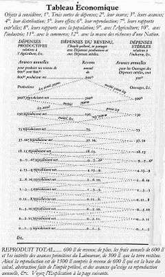
The Tableau économique (Economic Table) of François Quesnay (1758), which laid the foundation of the Physiocrat school of economics is credited as the "first precise formulation" of interdependent systems in economics and the origin of multiplier theory.^[3] In the tableau économique, one sees variables in one period (time t) feeding into variables in the next period (time t+1), and a constant rate of flow yields geometric series, which computes a multiplier.

The modern theory of the multiplier was developed in the 1930s, by Kahn, Keynes, Giblin, and others,^[4] following earlier work in the 1890s by the Australian economist Alfred De Lissa, the Danish economist Julius Wulff, and the German-American economist N. A. J. L. Johannsen.^[5]

Critiques

Economist Robert Barro believes that the Keynesian multiplier is close to zero. For every dollar the government borrows and spends, spending elsewhere in the economy falls by almost the same amount.^[6]

See also

• Complex multiplier
• Local multiplier effect
• Multiplier uncertainty
• Social Multiplier Effect

References

1. James Hamilton (1994), Time Series Analysis, Chapter 1, page 2. Princeton University Press.
2. Helmut Lütkepohl (2008), 'Impulse response function'. The New Palgrave Dictionary of Economics, 2nd. ed.
3. The multiplier theory, by Hugo Hegeland, 1954, p. 1
4. The Economic record, by the Economic Society of Australia and New Zealand, 1962, p. 74 Donald Markwell, Keynes and Australia, Reserve Bank of Australia, 2000, pages 34-7. http://www.rba.gov.au/publications/rdp/2000/pdf/rdp2000-04.pdf
5. The origins of the Keynesian revolution, by Robert William Dimand, p. 117
6. Cassidy, John (10 October 2011). "The Demand Doctor". The New Yorker. Retrieved 9 October 2011.