Regression validation
| Part of a series on Statistics |
| Regression analysis |
|---|
 |
| Models |
| Estimation |
| Background |
|
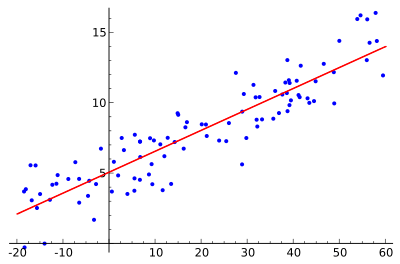
In statistics, regression validation is the process of deciding whether the numerical results quantifying hypothesized relationships between variables, obtained from regression analysis, are acceptable as descriptions of the data. The validation process can involve analyzing the goodness of fit of the regression, analyzing whether the regression residuals are random, and checking whether the model's predictive performance deteriorates substantially when applied to data that were not used in model estimation.
Validation using R2
An R2 (coefficient of determination) close to one does not guarantee that the model fits the data well, because as Anscombe's quartet shows, a high R2 can occur in the presence of misspecification of the functional form of a relationship or in the presence of outliers that distort the true relationship.
One problem with the R2 as a measure of model validity is that it can always be increased by adding more variables into the model, except in the unlikely event that the additional variables are exactly uncorrelated with the dependent variable in the data sample being used.
Analysis of residuals
The residuals from a fitted model are the differences between the responses observed at each combination values of the explanatory variables and the corresponding prediction of the response computed using the regression function. Mathematically, the definition of the residual for the ith observation in the data set is written
with yi denoting the ith response in the data set and xi the vector of explanatory variables, each set at the corresponding values found in the ith observation in the data set.
If the model fit to the data were correct, the residuals would approximate the random errors that make the relationship between the explanatory variables and the response variable a statistical relationship. Therefore, if the residuals appear to behave randomly, it suggests that the model fits the data well. On the other hand, if non-random structure is evident in the residuals, it is a clear sign that the model fits the data poorly. The next section details the types of plots to use to test different aspects of a model and gives the correct interpretations of different results that could be observed for each type of plot.
Graphical analysis of residuals
A basic, though not quantitatively precise, way to check for problems that render a model inadequate is to conduct a visual examination of the residuals (the mispredictions of the data used in quantifying the model) to look for obvious deviations from randomness. If a visual examination suggests, for example, the possible presence of heteroskedasticity (a relationship between the variance of the model errors and the size of an independent variable's observations), then statistical tests can be performed to confirm or reject this hunch; if it is confirmed, different modeling procedures are called for.
Different types of plots of the residuals from a fitted model provide information on the adequacy of different aspects of the model.
- sufficiency of the functional part of the model: scatter plots of residuals versus predictors
- non-constant variation across the data: scatter plots of residuals versus predictors; for data collected over time, also plots of residuals against time
- drift in the errors (data collected over time): run charts of the response and errors versus time
- independence of errors: lag plot
- normality of errors: histogram and normal probability plot
Graphical methods have an advantage over numerical methods for model validation because they readily illustrate a broad range of complex aspects of the relationship between the model and the data.
Quantitative analysis of residuals
Numerical methods also play an important role in model validation. For example, the lack-of-fit test for assessing the correctness of the functional part of the model can aid in interpreting a borderline residual plot. One common situation when numerical validation methods take precedence over graphical methods is when the number of parameters being estimated is relatively close to the size of the data set. In this situation residual plots are often difficult to interpret due to constraints on the residuals imposed by the estimation of the unknown parameters. One area in which this typically happens is in optimization applications using designed experiments. Logistic regression with binary data is another area in which graphical residual analysis can be difficult.
Serial correlation of the residuals can indicate model misspecification, and can be checked for with the Durbin–Watson statistic. The problem of heteroskedasticity can be checked for in any of several ways.
Out-of-sample evaluation
Cross-validation is the process of assessing how the results of a statistical analysis will generalize to an independent data set. If the model has been estimated over some, but not all, of the available data, then the model using the estimated parameters can be used to predict the held-back data. If, for example, the out-of-sample mean squared error, also known as the mean squared prediction error, is substantially higher than the in-sample mean square error, this is a sign of deficiency in the model.
See also
References
- Kmenta, Jan (1986). Elements of Econometrics (Second ed.). New York: Macmillan. pp. 593–600. ISBN 0-02-365070-2.
External links
- How can I tell if a model fits my data? (NIST)
- NIST/SEMATECH e-Handbook of Statistical Methods (Accessed September 2011),
![]() This article incorporates public domain material from the National Institute of Standards and Technology website http://www.nist.gov.
This article incorporates public domain material from the National Institute of Standards and Technology website http://www.nist.gov.