Representations of the atmospheric boundary layer in global climate models
Representations of the atmospheric boundary layer in global climate models play a role in simulations of past, present, and future climates. Representing the atmospheric boundary layer (ABL) within global climate models (GCMs) are difficult due to differences in surface type, scale mismatch between physical processes affecting the ABL and scales at which GCMs are run, and difficulties in measuring different physical processes within the ABL. Various parameterization techniques described below attempt to address the difficulty in ABL representations within GCMs.
What is the ABL?
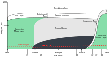
The ABL is the lowest part of the Earth's atmosphere, the troposphere. The ABL is the only part of the troposphere in contact with the Earth's surface, so the ABL is directly affected by forcings originating at the surface.[1] Such forcings include: heat flux, moisture flux, convection, friction, pollutant emission, and topographically modified flow. Response times to these forcings typically are an hour or less.[1]
Why is modeling of the ABL so difficult?
Surface forcings must be accounted for in GCMs in order to have accurate simulations of the Earth's climate. Unfortunately, difficulty in simulating these forcings arise for a number of reasons. First, the Earth's surface is not uniform. It consists (broadly) of land, water, and ice, and each surface interacts differently with the atmosphere. Secondly, the time and spatial scales for forcings between the Earth's surface and atmosphere occur on scales much less than the scales at which GCMs are run. Third, many of these processes are difficult to measure directly. So, these forcings need to be parameterized as a result.[2]
In general, the Earth is divided into a 3-D grid. Prognostic equations for each relevant physical process are run for each grid point. From there, grid point values for each variable are interpolated into each grid cell, which can then be analyzed.[2]
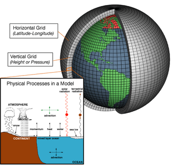
Grid resolution for GCMs varies considerably, on the order of 1 to 5 degrees (approximately 110 to 550 km for latitude, up to 110 km for longitude) in the horizontal, and 10 levels in the vertical. As grid resolution increases, the amount of computational time needed to run the model increases exponentially, because there are many more grid points comprising the model. Furthermore, even with the highest resolution of 1 degree, the spatial scales of many of the physical processes incorporated in the model are still far smaller than the model resolution.[2]
GCM cloud parameterizations
Clouds and convection often arise from small-scale processes that occur within the ABL. Additionally, clouds and convection help tie together the ABL with the free atmosphere, as convection helps grow the ABL. Furthermore, when the environment is sufficiently unstable, convection may help wash away the temperature inversion that caps the ABL. Also, "the convective motions associated with clouds produce important fluxes of mass, momentum, heat, and moisture".[2] The scales at which these fluxes are set come about are usually much smaller than GCM grids. However, these fluxes are often greater than those of the synoptic flow. Parameterizations of clouds and convection aim to address the scaling differences between GCM grids and cloud/convective scales.[2]
GCM cloud parameterizations account for at least two cloud types: convective clouds and large-scale supersaturation clouds. "Large-scale supersaturation clouds occur when the relative humidity in a grid box at some model level exceeds a critical value".[2] One way of accounting for large-scale supersaturation clouds is by setting the critical relative humidity value to 80%, assigning grid boxes with relative humidity values at or above 80% as cloud covered. Another way to account for large-scale supersaturation clouds is to benchmark clouds via temperature variability, in that wherever the temperature "causes the relative humidity to reach 100% is cloud covered".[2]
Moist adiabatic adjustment scheme
Convective clouds follow one of three general parameterization schemes. The first scheme is moist adiabatic adjustment. The main advantage of this method is that it is simple, in that if the moist adiabatic lapse rate is exceeded, moisture and heat within the vertical layer are adjusted so that air within the layer is saturated.[2][3] In turn the lapse rate is then adjusted to the moist adiabatic lapse rate, conserving energy, raining out excess moisture while not transporting momentum. The disadvantage of this scheme is that it over-estimates convection, as constrains an entire grid box to act in a convective manner, unrealistic in the real atmosphere.[2]
Kuo scheme
The second scheme is the Kuo parameterization, and is more complex than the moist adiabatic adjustment scheme.[2][3] This scheme is concerned with large-scale moisture convergence as the moisture source for convection. A weakness of this scheme is convective heating, in that this parameterization scheme assumes that convection heats by mixing cloud and environmental air, instead of heating produced by subsidence between clouds.[2]
Arakawa-Schubert scheme
The Arakawa-Schubert scheme is the third scheme, and is the most comprehensive.[2][3] This scheme models cumulus cloud/environment interactions, entrainment and detrainment of air/moisture, cloud downdrafts, and subsidence outside of clouds. Additionally, this scheme assumes quasi-equilibrium, with cloud dissipation at a "rate sufficient to keep the atmosphere near equilibrium in the face of large-scale destabilization."[2]
Turbulence closure
Most atmospheric turbulence occurs within the ABL, whereas the free atmosphere is largely non-turbulent. So, in order to have a proper accounting for motions within the ABL, GCMs must properly account for turbulence within the ABL. To do this, GCMs must have some way of achieving turbulence closure.
Turbulent processes can be roughly combined into three categories: heat flux, moisture flux, and momentum flux.[2] When calculating these fluxes, one ends up with more unknowns than equations, which means those equations cannot be solved directly. In order to calculate turbulent fluxes and close the equations, one must make parameterizations for the higher order terms. The sections below describe methods for parameterizing turbulent fluxes and turbulence closure.
Local and non-local closure
There are two methods of parameterizing turbulent fluxes. The first is local closure. Local closure ties the unknown turbulent quantity at a specific point in space to values and gradients of known quantities at the same point. Additionally, local closure likens turbulent transport to molecular diffusion, and is usually first or second order.[1]
The second method of parameterizing turbulent fluxes is nonlocal closure. Turbulence does not just depend on local values and gradients due to the superposition of many individual eddies. Unlike local closure, nonlocal closure links unknown turbulent quantities to known quantities at many points in space.[1]
K-theory
K-theory (eddy diffusivity/viscosity theory) is a form of local closure, and is the main first order closure scheme within the surface layer. K-theory follows a similar concept as molecular viscosity, in that the turbulent flux of a quantity is proportional to its spatial gradient, with K as the eddy viscosity/diffusivity. K-theory is powerful because the flux of quantities can be directly tied into the gradient of the mean quantities with height, multiplied by a value K. The idea behind K-theory is that turbulence eliminates gradients, creating a net flow of quantities down their gradients.[1] So K is positive.
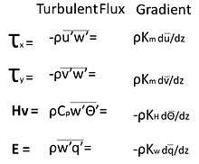
The eddy diffusivity/viscosity equations are shown in the figure on the right. Km represents eddy viscosity, while KH and KW represent eddy diffusivity of heat and moisture, respectively. τx and τy represent Reynolds stress (momentum flux) in the x and y directions, Hv represents the turbulent heat flux, and E represents the turbulent moisture flux. ρ is the density of air, u', v', and w' are velocity perturbations, and θ' and q' are potential temperature and moisture perturbations. Other key points regarding K:[1]
- K = 0 when flow is laminar
- K = 0 at the surface
- K increases as TKE (turbulent kinetic energy) increases
- K varies with static stability
- K is non-negative, with turbulent fluxes flowing down-gradient
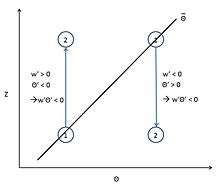
K-theory is best applied in statically neutral environments, with predominately mechanically-generated turbulence, though it has been applied to statically stable environments.[1] The figure to the right demonstrates how temperature flux works in a stable environment. If a parcel is displaced upward in a stable environment, w' is positive 0, and θ' is greater than the mean θ. So w'θ' is greater than zero. Conversely, when a parcel is displaced downward, w' is negative, and θ' is negative.
Depending on the vertical resolution of the model, K-theory may be used to account for the various fluxes within the ABL.[2][3] Additionally, K-theory can be applied in unstable conditions within the mixed layer if a counter-gradient term is applied, which accounts for buoyancy-driven turbulence.
Bulk aerodynamic formulae
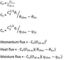
As an alternative to K-theory, ABL fluxes can be accounted for through the use of bulk aerodynamic formulae.[2]
The bulk aerodynamic formulae use Cd, Ch, and Cq, where Cd is the drag coefficient, Ch is the heat exchange (transfer) coefficient, and Cq is the moisture exchange (transfer) coefficient.[3] Each of these coefficients are functions of the known variables, such as the average wind speed at 10m, and average potential temperature and moisture at the surface and 10m. Additionally, each of these coefficients varies based on stability. From the known variables the exchange coefficients can be easily calculated, and thus, the fluxes can be easily calculated as well. The image below shows the equations used for calculating the exchange coefficients and fluxes, with u* as the frictional velocity.[1]
References
- 1 2 3 4 5 6 7 8 Roland B. Stull, ed. (1988). An introduction to boundary layer meteorology. 13. Springer. pp. 2, 200, 204, 208, 261–269.
- 1 2 3 4 5 6 7 8 9 10 11 12 13 14 15 16 Hartmann, Dennis L. (1994). Global physical climatology. 56. Academic press. pp. 257–258, 260–263.
- 1 2 3 4 5 Kalnay, Eugenia (2003). Atmospheric modeling, data assimilation and predictability. Cambridge University Press. pp. 130–135.